Quantum mechanics
Table of Contents
- 1. Abbreviations
- 2. Information loss
- 3. Math - Trigonometry
- 4. Linear algebra (vectors)
- 5. Calculus
- 6. Fields
- 7. Complexe getallen
- 8. Identity
- 9. Translation / symmetry
- 10. Poisson bracket (PB)
- 11. Fysica - Momentum
- 12. Hamiltonian
- 13. Electromagnetism
- 14. Quantum mechanics
- 14.1. Basis
- 14.2. Hilbert space
- 14.3. Quantum mechanical spin
- 14.4. Qubit
- 14.5. Wavefunction
- 14.6. "Preparing" a system
- 14.7. Eigenvector vergelijking
- 14.8. Pauli matrices
- 14.9. Matrix
- 14.10. <A|M|B>
- 14.11. Hermitic operator
- 14.12. Kronecker product
- 14.13. Schrodinger
- 14.14. Commutator
- 14.15. Heisenberg
- 14.16. Projectie-operator
- 14.17. Density matrix
- 14.18. Entanglement
- 15. Strange quantum effects
- 16. Verwijderd
1 Abbreviations
https://www.caam.rice.edu/~heinken/latex/symbols.pdf https://www.rapidtables.com/math/symbols/Basic_Math_Symbols.html C-c-x-l
https://github.com/apprenticeharper/DeDRM_tools/releases/tag/v7.2.1
1.1 Tekens
| <Q> | average outcome of entity Q when repeating an experiment, Dirac brackets |
| \(\{\}\) | mathmatical set, e.g. set of all position vectors (in a system) |
| \(∫\) | integral |
| \(\sum \limits_{a,b}\) | alle mogelijke combinatie van a met b (bijv. u en d, samen 4) |
| \(f(x)\mid _a^b\) | delta of a function when substituting a and b |
| \(\mid A\rangle\) | ket (vector), e.g. column vector with complex numbers \(\alpha_1\) to \(\alpha_n\) |
| non-capital: eigenstate | |
| \(< A \mid B >\) | inner product of A and B (bra[c]ket) |
| \(< B \mid\:\) | bra B |
| \(\cdot\) | inner product (lineair algebra, logical AND, multiplication |
| \(\dot{x}\) | derivative of x (in time) |
| \(x'\) | derivative of x (in time) |
| coordinaat na translatie | |
| \(x’’\) | second order derivative (in time) |
| * | conjugaat |
| \(\nabla\) | nabla, del; divergence, derivative of a field |
| → | active transformatie |
| [] | m = [mass] = [kg] |
| \(\vec{u}\) | vector: object met richting en grootte; ook wel (x,y,z), 3(d)-vector |
| \(a\vec{u}\) | vector multiplication: a is called a scalar (normal number in relation with vector |
| negative \(a\) means the opposite direction | |
| \(\vec{u}+\vec{w}\) | vector addition: adding start of arrow to end of arrow |
| \(\hat{u}\) | (accent circonflex) unit vector u – vector with unit length 1 |
| \(\parallel u \parallel\) | norm / size of vector u |
| or \(\mid u \mid\) | |
| \(\vec{f}_{ij}\) | force acted by j on i |
| \(\alpha_1\) | component 1 of ket A |
| \(\partial\) | delta van een partiele derivaat (is een differentiaal, zie plaatjes hieronder) |
| \(\delta\) | \(\delta_{ij}\) Kronecker delta: is 0 als i≠j en 1 als i=j |
| εijk | 0 is two subscript are identical, -1 if counterclockwise and 1 if clockwise |
1.2 Griekse letters
| \(σ_x\) | x-component van 3-vector operator σ, is niet eenvoudig inwendig product: qubit |
| σ | two-bit state, 3-vector operator, spin |
| θ | hoek met x-as (evt. in complexe vlak) |
| A | stelling of apparaat of ket |
| C | ket |
| Det H | determinant in a Hessian matrix |
| F | integral of function f |
| H | Hessian matrix |
| infinitesimaal | |
| δA=0 is een afkorting van δA/dxi = 0 bij functie A(x,y) | |
| gemiddeld wel: \(<σx>\) | |
| 1 of 1,2,3 | x,y,z |
| ψ and φ | vaak gebruikt als aanduiding van een state als time evolution belangrijk is |
1.3 Letters
| a | versnelling |
| ab | subscript is een index, array: verschillende exemplaren met zelfde letter aangeduid |
| 1,2,3 of variabele: i,j,k, of component 3-vector operator zijn: x,y,z | |
| c | constante (bijv. lichtsnelheid) |
| d | differentiaal, een delta in de limiet naar 0 |
| e | Euler getal: 2,7…., \((e^n)’ = e^n\) |
| ei | orthogonal unit axis |
| lim | limiet, zie differentiaal |
| f | functie f, zie ook fij |
| f(x) | functie f levert een waarde voor f gegeven x op |
| g | “een tweede functie”, zwaartekrachtconstante (Aardse constante), |
| i | imaginary number: i2 = -1; all axes (see i,j,k) |
| often the associated summation sign is left out | |
| i,j,k | orthogonal unit vectors (along the axes x,y,z) |
| \(\hat{i}, \hat{j}, \hat{k}\) | orthogonale unit vectors die assenstelsel definieren, of ei (indien xi de assen) |
| log | logaritme, log10(1000)=3, of bij x=ay is y=alog (x) |
| ln | ^{e}log |
| m,n | willekeurige assen/vectoren |
| m | massa |
| p | momentum |
| \(q_i\) | algemene coordinatensysteem, niet per se Carthesiaans |
| r | straal; positievector, dus vector van origo naar punt x,y,z |
| t | tijd |
| tan-1 | omgekeerde tangens in bereik (-π/2, π/2), syn: arctan, boogtan, atan, bgtan |
| v | snelheid |
| x,y,z | coordinaten of assen in 3D-ruimte |
| xi | de drie coordinaten tezamen genoteerd, positie |
| z,w | complex getal |
1.4 numbers
- natural (N): {1,2,3, …}, soms nul
- integers (Z, zahlen): ook negatief en nul
- rational (Q): quotient
- real (R): alle punten op lijn
- irrational: wel real, niet rational
- complex (C)
- hypercomplex, bijv. quaternionen (H)
1.5 Engels
- expanding to the first order = afgeleide bepalen
2 Information loss
- "minus one law"
- distinctions are conserved
- if two identical systems start out in a different state, they stay different, and, were always different
- the time evolution of states "must have one arrow in and one arrow out"
- quantum version: unitarity
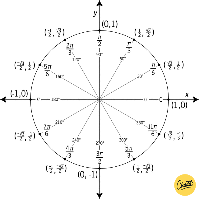
3 Math - Trigonometry
(cosinus, sinus)
4 Linear algebra (vectors)
- nomenclature
- linear algebra = linear combinations of vectors
- scalar = normal number in relation with a vector
- vector space
- een soort array (en niet een 3-vector)
- abstract
- kan van alles bevatten: integer, real, complex getal, complexe vectoren etc, en zelfs functies
- kan ieder aantal dimensies hebben
- may or may not have anything to do with space
- orthonormal basis (unit length and a right angles to each other) can be used to describe a vector
- pro: math can be made explicit
- con: vectors / operators and their relations are in reality independent from the arbitrary basis, that insight is lost
- components: \(\vec{V} = V_x\hat{i} + V_y\hat{j} + V_z\hat{k}\), or vector v in N-dimensional space with orthonormal basis e: \(v = v_1 e_1 + v_2 e_2 ... + v_n e_n \equiv \sum \limits_{k=1}^n v_k e_k\)
- multiplication with a scalar (result: vector)
- determining norm
- length or size or distance
- \(\parallel \: a \parallel = \sqrt{a^2_1 + a^2_2 + a^2_3} = \sqrt{a \cdot a}\)
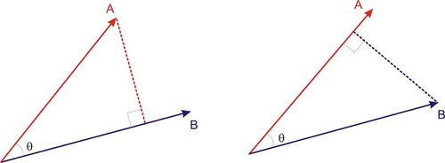
- inner product (result: scalar)
- = scalar product, inproduct, dot product (in case of non-complex vectors)
- \(uv = \parallel u \parallel \parallel v \parallel cos(\theta)\)
- \(uv = u_x v_x + u_y v_y + u_z v_z\)
- \(uv = uv^T\) vanwege de matrixrekenregels
- betekenis
- de componenten van een vector zijn het inwendige product met de basisassen
- met inwendig product kun je hoek berekenen van vectoren
- wat is het? https://www.sharetechnote.com/html/Handbook_EngMath_Matrix_InnerProduct.html
- hoe reken je met matrixen? https://samenvattingen.inter-actief.utwente.nl/images/8/88/MatchC1_-_samenvatting.pdf
- waarom zo rekenen? https://www.embedded.com/why-multiply-matrices/
- cross product \(\times\) (result: vector)
- \((\vec{V} \times \vec{A})_x = V_yA_z - V_zA_y\), etc for y and z
- or, \((\vec{V} \times \vec{A})_i = \sum \limits _k \sum \limits _j \epsilon_{ijk} V_j A_k\)
- result: vector perpendicular to both vectors with the length being the area of the parallelogram that results from both starting at the same spot, thus zero is they are (anti-)parallel or if one of them is zero
- curl: suppose the vector field describes the velocity field of a fluid flow (such as a large tank of liquid or gas) and a small ball is located within the fluid or gas (the centre of the ball being fixed at a certain point). If the ball has a rough surface, the fluid flowing past it will make it rotate. The rotation axis (oriented according to the right hand rule) points in the direction of the curl of the field at the centre of the ball, and the angular speed of the rotation is half the magnitude of the curl at this point. The curl of the vector at any point is given by the rotation of an infinitesimal area in the xy-plane (for z-axis component of the curl), zx-plane (for y-axis component of the curl) and yz-plane (for x-axis component of the curl vector).
5 Calculus
5.1 Infinitesimal change
- \(\delta\) is a non-real (hyperreal) infinitesimal (higher than zero and lower than the lowest real number)
- \(\epsilon\) is a real number used in connection with small changes (but not always small)
- \(d\) or \(dx\) in \(df/dx\) is not something you can calculate independently with: in the limt of the definition of a differential it can become very small
- \(x \rightarrow x + y\delta\)
- \(\dot{x} \rightarrow \dot{x} + \dot{y}\delta\)
- \(\delta x = y \delta\)
- \(\delta \dot{x} = \dot{y}\delta\)
- \(\delta x = \epsilon f_x = \epsilon y\) (en y=$fx(x) in which the function calculates the change)
- \(\delta \dot{x} = \epsilon \dot{f}(x)\)
- thus, \(\frac{df(x)}{dx} = \frac{\delta f(x)}{\epsilon}\) in which \(\epsilon\) is a small distance
5.2 Partial differentiation
- How to
- \(F = x^2 + xy + y^2\)
- \(\frac{\partial F}{\partial x} = 2x + y\)
- Time derivative of a multivariable function: see Poisson Bracket
- For the change z(x+Δx,y+Δy)−z(x,y) of the function z(x,y) bacause of a small change Δx and Δy: z(x+Δx,y+Δy) − z(x,y) ≈ z′x(x,y)Δx + z′y(x,y)Δy.
- The changes in x and/or y have to be small to guarantee a good approximation.
- Meaning: ∂z/∂x is actually ∂z(x,y)/∂x as the derivative depends on the coordinates
- Important rules
- \(\frac{\partial q}{\partial p} = 0\)
- \(\frac{\partial F}{\partial p} \frac{\partial H}{\partial q} = 0\)
- here you can exchange p and q: \(\frac{\partial}{\partial p} \frac{\partial H}{\partial q}\)
6 Fields
- types: scalar (temperature) and vector fields (speed)
- \(\vec{\nabla}\) - nabla, can never stand alone, derivative symbol for fields: \(\nabla_x \equiv \frac{\delta}{\delta x}\); see example below
- vector field
- \(\vec{\nabla} \cdot (\vec{\nabla} \times \vec{A})=0\) (divergence of a curl, proof)
- moreover, a divergence is only zero if it is the curl of a field
- \(\vec{\nabla} \times (\vec{\nabla}T(x))=0\) (divergence of a gradient, proof)
- inner product with nabla (result: scalar): derivative ("divergence")
- \(\vec{\nabla} \cdot \vec{A} = \frac{\delta A_x}{\delta x} + \frac{\delta A_y}{\delta y} + \frac{\delta A_z}{\delta z}\)
- cross product with nabla: curl, rotation of a field
- \((\vec{\nabla} \times \vec{A})_x = \frac{\delta A_z}{\delta y} - \frac{\delta A_y}{\delta z}\), etc. for y and z
- or, \((\vec{\nabla} \times \vec{A})_i = \sum\limits_k \sum \limits _i \epsilon_{ijk} \frac{\delta A_k}{\delta x_j}\)
- scalar field
- derivative (result: vector): gradient
- \(\nabla_xT \equiv \frac{\delta T}{\delta x}\), etc for y and z.
- derivative (result: vector): gradient
6.1 Divergence
6.1.1 analogy to irreversibility
- a volume of infinite dots in phase space, uniformly dispersed
- following their Hamiltonian energy surfaces H(q,p) that the phase space like layers
- number of dimensions is 2N-1 dimensions (subtracting 1 for energy)
- reversibility requires the absence of convergence and divergence, the joining of creation of new layers, or if the points have a fixed volume: an increase or decrease of volume (incompressibility)
6.1.2 3d model
- fluid current in 3d: a speed vector field \(\vec{v}(x,y,z)\)
- for now no time dependence: a stationary speed field
- the net flow into a small box across two opposing faces is proportional to \(-\frac{\partial v_x}{\partial x}\:dx\:dy\:dz\)
- the change in \(v\) over face \(x=c\) and \(x=c+delta\) at about \((c_x,c_y,c_z)\) is \(\partial x_x\)
- this results in the change in speed per distance (\(\frac{m}{sm}\))
- multiply by \(\delta x\) to get the change in speed (over a line)
- multiply by \(\delta y\delta x\) to obtain a flow in a small volume around the line (in volume/time, \(\m^3/s\))
- across all faces \(-(\frac{\partial v_x}{\partial x}\frac{\partial v_y}{\partial y}\frac{\partial v_z}{\partial z})\:dx\:dy\:dz\)
6.1.3 divergence \(\nabla\)
- definition: \(\nabla \cdot \vec{v} = (\frac{\partial v_x}{\partial x} + \frac{\partial v_y}{\partial y} + \frac{\partial v_z}{\partial z})\)
- if a field is incompressible: divergence is zero
6.1.4 Liouville's theorem
- in phase space the dimensions double
- 1. divergence in phase space: \(\nabla \cdot \vec{v} = \sum{( \frac{\partial v_{q_i}}{\partial {q_i}} + \frac{\partial v_{p_i}}{\partial {p_i}})}\)
- 2. alternative way formulated: \(v_{q_{i}} = \dot{q}_i\) en \(v_{p_{i}} = \dot{p}_i\)
- joining 1 and 2: \(\nabla \cdot \vec{v} = \sum{( \frac{\partial}{\partial q_i} \frac{\partial H}{\partial q_i}- \frac{\partial}{\partial p_i} \frac{\partial H}{\partial {q_i}})} = 0\)
- therefore, there is no divergence if the system satisfies Hamilton’s equations
- rephrasing: a volume of phase space is conserved with time
- in quantum machanics: unitarity
7 Complexe getallen
- consists of two real numbers
- \(z = x + iy\) complex getal in Carthesiaans complex vlak en in componentenvorm
- \(z = re^{iθ} = r (cos \: θ + i \: sin \: θ)\) polar representation
- adding (and subtracting) is adding components: second "vector" is added to first
- imaginary multiplication: (r1eiθ1)(r2eiθ2) = (r1 r2)(ei(θ1+θ2))
- multiplication lead to rotation: the first "vector" is rotated by the angle that the second "vector" has with the real axis
- why? https://betterexplained.com/articles/a-visual-intuitive-guide-to-imaginary-numbers/
7.1 Complex vector
- ket-vector or ket
- |A> is a complex vector (in a complex vector space, or "ket-space")
- vectors are not written with a hat but with a capital
- rule of multiplication with a complex number: z|A> = |zA> = |B>
- addition and multiplication of complex vectors is possible if the number of dimensions match
- |A> + |B> = |C>
- |A> + |B> = |B> + |A>
- |A> + 0 = |A>
- |A> + (-|A>) = 0
- {|A> + |B>} + |C> = |A> + {|B> + |C>}
- z{|A> + |B>} = z|A> + z|B>
- {z + w} |A> = z|A> + w|A>
- rules for calculatig with kets and column vectors: p.25
- |A> is either
- complex valued function
- column vector of complex numbers which are the components in a orthonormal basis
7.1.1 complex vector as column vector
- \(|A \rangle = \left( \begin{array}{c} z_1 \\ z_2 \end{array} \right)\) indien |A> twee dimensies heeft
- \(z\left( \begin{array}{c} \alpha_1 \\ \alpha_2 \end{array} \right) = \left( \begin{array}{c} z\alpha_1 \\ z\alpha_2 \end{array} \right)\)
- \(\left( \begin{array}{c} \alpha_1 \\ \alpha_2 \end{array} \right) + \left( \begin{array}{c} \beta_1 \\ \beta_2 \end{array} \right) = \left( \begin{array}{c} \alpha_1 + \beta_1 \\ \alpha_2 + \beta_2 \end{array} \right)\)
- \(|A \rangle = \sum \limits_i \alpha_i | i \rangle\) decomposes the vector in components
- i is an orthonormal basis of ket-vectors
- the label i is confusingly different: there (probably?) is an \(i_i\)
- components can be calculated by calculating the inner product with the basis vectors:
- \(\langle j | A \rangle = \sum \limits_i \alpha_i \langle j | i \rangle\): inner product with basis bra j
- imagine the subscript \(i_i\) and realize \(j = i_j\)
- \(\langle j | A \rangle = \delta_{ij}\) ⇒ \(\langle j | A \rangle = \alpha_j\)
- \(| A \rangle = \sum \limits_i | i \rangle \langle i | A \rangle\): fill in the last equation in the starting equation
- \(\langle j | A \rangle = \sum \limits_i \alpha_i \langle j | i \rangle\): inner product with basis bra j
7.2 Conjugation
- dual version of complex number or vector: negating imaginary part
- and it transforms a column vector to a row vector and vice versa
- the conjugation sign is *
- it allow the formation of bra-kets which is required for (and is the sign of) the inner product and squaring (e.g. to go from probaility amplitude to probability)
- \(z* = x-iy = re^{-iθ}\)
- ( |A> )* = <A|, or, a bra becomes a ket
- { |A> + |B> }* = <A| + <B|
- ( z|A> )* = <A|z*
- ( <A|B> )* = <B|A>
- <A| = \((z_1^*, z_2^*)\), as in, a column becomes a row
- \(z^* z = r^2\)
- "a real number is equal to its complex conjugate", \(\lambda = \lambda^*\)
7.3 Inner product
- <A|Z> = \(ɑ^*_1 z_1 + ɑ^*_2z_2\) (result: complex number)
- <A|A> = 1 if vector A normalised (unit vector for 3-vectors)
- <A|B> = 0 means A and B are orthogonal
- <C| { |A> + |B> } = <C|A> + <C|B>
- squaring inner product \(| \langle A | B \rangle |^2 = \langle A | B \rangle \langle B | A \rangle\) to negate the imaginary part
7.4 Phase factor
- complex numer with radius 1
- \(z^* z = 1\)
- \(z = e^{iθ} = \cos(θ) + i\sin(θ)\)
8 Identity
- elements that leaves the set that operation is applied on unchanged
- multiplicaton: 1, addition: 0
- nxn-matrix: identity matrix I met 1-en op symmetrie lijn en verder nullen
- als \(U^\dagger U = I\) dan \(U\dagger = U\)
9 Translation / symmetry
- in case of translation invariance
- momentum is conserved
- Poisson Bracket can be used to generate an equation of motion through derivatives
10 Poisson bracket (PB)
10.1 derivation
- consider F(q,p)
- a function of a point in phase
- in case of following a trajectory in phase space: a function of time
- time derivative of F: \(\dot{F} = \sum {(\frac{\partial F}{\partial q_i} \dot{q}_i + \frac{\partial F}{\partial p_i} \dot{p}_i)}\), as
- derivative of t: \(\dot{q}\) = \(\dot{q}(t)\)
- derivative of q: \(\frac{\partial F}{\partial q} = \frac{\partial F(q,t)}{\partial q}\)
- chain rule of two independent variables: \(\frac{\partial F(q,p)}{\partial t} = \frac{\partial F(q,p)}{\partial q}\frac{\partial q}{\partial t} +\;\)…
- over the complete range of t \(\dot{q}\) gives the time derivative of q which is entered as \(\partial q\) into \(\frac{\partial F}{\partial t}\) at (q,p)
- filling in the Hamiltonian equations: \(\dot{F} = \sum {(\frac{\partial F}{\partial q_i} \frac{\partial H}{\partial p_i} - \frac{\partial F}{\partial p_i} \frac{\partial H}{\partial q_i})} = \{F, H\}\)
- effect of adding something else than A or B
- if A and B do not contain p or q the PB is zero
- adding \(q(t)\) or \(p(t)\)
- \(\{q_k, H\} = \frac{\partial H}{\partial p_i} = \dot{q_k}\) (the PB contains the Hamiltonian), because \(\frac{\partial q}{\partial q}\) = 1 en \(\frac{\partial q}{\partial p} = 0\)
- \(\{p_k, H\} = \frac{\partial H}{\partial q_i} = \dot{p_k}\) (now without negative sign in the Hamiltonian equation of motion)
- \(\{q_i,q_j\} = 0\) en \(\{p_i,p_j\} = 0\) as i and j differ and are independent
- \(\{q_i, p_j\} = \delta _{ij}\)
- \(\{q^n,p\}=\frac{d(q^n)}{dq}\) (provable through mathematical induction)
- \(\{F(q,p),p_i\} = \frac{\partial F(q,p)}{\partial q_i}\)
- \(\{F(q,p),q_i\} = -\frac{\partial F(q,p)}{\partial p_i}\)
10.2 definition
- Poisson bracket: \(\{A, B\} = \sum {(\frac{\partial A}{\partial q_i} \frac{\partial B}{\partial p_i} - \frac{\partial A}{\partial p_i} \frac{\partial B}{\partial q_i})}\)
10.3 function and examples
- \(\{p \vee q \vee f(p,q), H\} = \dot{p}\) bij p – the PB of something (q, p, or a function of [one of] them) and the Hamiltonian, is its time derivative
- \(\{F(p,q), p \vee q\} = \frac{\delta F}{\delta q}\) bij p – the PB of a function with \(p_i\) has the effect of differentiating the function with respect to \(q_i\), with q vice versa but with negative sign
- \(\{p \vee q, Q\} = \dot{p}\) bij p and $\{Qi, Qj\}$– the PB of a coordinate or momentum with a conserved quantity gives the transformation behavior of it under a symmetry
- e.g. angular momentum: to compute the change in any quantity (or just p and q?) when the coordinates are rotated (under a symmetry) about the i-th axis, we compute the Poisson bracket of the quantity with the angular momentum with \(\delta F = \{F, L_i\}\), to that it is proportional, in which F is "any quantity" see example
- second, \(\{L_x\, L_y\} = L_z\), ofwel \(\{L_i, L_j\} = \sum\limits{k}\epsilon_{ijk} L_k\), see 11.2.2 for an example
- transformation on a line (repeat 2): in case of translation invariance / symmetry, \(\{F(x),p\} = \frac{dF}{dx} \Rightarrow \delta F = \epsilon \{F(x),p\} = \epsilon \frac{dF}{dx}\)
- small change in a quantity under a time-transformation (repeat 1): \(\{p, H\} = \dot{p'} = \frac{\delta p}{\epsilon}\) where \(\epsilon\) is the time-transformation
- generator G(p,q) invullen als variant op de Hamiltoniaan
- \(\delta q_i = \{q_i, G\}\)
- aangezien de Hamiltoniaan ook een funcie met p en q is
- indien E van systeem gelijk blijft na deze transformatie (waar ook uit gevoerd) gaat het om transformatie binnen een symmetrie
- eis is derhalve {H, G} = 0, in other words, H does not change with a transformation by G
- derhalve ook {G, H} = 0 so G is conserved
10.4 axiomatic rules
- \(\{A,C\} = -\{C,A\}\) (antisymmetry), therefore \{A,A\} = 0$
- \(\{kA,C\} = k\{A,C\}\) en \(\{(A+B),C\} = \{A,C\} + \{B,C\}\) (antilinearity)
- \(\{(AB),C\} = B\{A,C\} + A\{B,C\}\)
11 Fysica - Momentum
11.1 Canonical momentum
- synonyms: conjugate momentum
- in comparison with mechanical momentum
- not per se gauge invariant
- not "real" / observable
11.2 Angular momentum
- mathmatical representation of a circle with radius
- \(x = r\:cos\:\theta\)
- \(y = r\:sin\:\theta\)
- mathmatical representation with carthesian coordinates
- \(x = x \: cos \: \theta + y \: sin \: \theta\)
- \(y = -x \: sin \: \theta + y \: cos \: \theta\)
- for a small angle:
- \(sin \: \delta = \delta\)
- \(cos \: \delta = 1 - \frac{1}{2} \delta^2 = 1\) which vanishes compared with the sinus
- infinitesimal rotation
- \(\delta x = \epsilon f_x = + \epsilon y\) and \(f_x = y\) and \(\delta\dot{x}=y\delta\)
- \(\delta y = \epsilon f_y = - \epsilon x\) and \(f_y = -x\) and \(\delta\dot{y}=-x\delta\)
- \(L = \frac{m}{2}(\dot{x}^2+\dot{y}^2)-V(x^2+y^2)\) Lagrangian for a particle in orbit
- \(Q = \sum\limits_{\:\:i}{p_if_i(q)}\) ⇒ \(Q = p_x f_x + p_y f_y\) if the rotation is invariant with respect to the Lagrangian
- \(L = xp_y - yp_x\) in which L is the angular momentum, to visualize
- \(L\) is invariant
- both \(p_i\) and \(x,y\) change with the rotation predictably
- using \(m=1\) \(p\) changes to \(v\): and \(v\) and \(x,y\) are easily visualized
- so a circling particles changes its momentum components continously, dependent on its coordinates on the circle
11.2.1 "3d" circle - Poisson bracket as generator of symmetry
- angular momentum is a vector \({\vec{L}}\) along the axis that rotates
- add \(\delta z = 0\) to the above and it rotates around the z axis
- components of \(\vec{L}\)
- \(L_z = xp_y - yp_x\) angular momentum as above (with the "viewing direction" parallel to the z axis
- \(L_x = yp_z - zp_y\) angular momentum, if the system is rotationally symmetric around the axis
- \(L_y = zp_x - xp_z\) angular momentum, …
- \(\{x,L_z\} = \{x, (x p_y - y p_x)\} = -y \sim \delta x\)
- \(\{x,L_z\} = \{y, (x p_y - y p_x)\} = x \sim \delta y\)
- \(\{z,L_z\} = \{z, (x p_y - y p_x)\} = 0 \sim \delta z\)
- or, \(\{x_i, L_j\}=\sum\limits_{\:k}\epsilon_{ijk}x_k\) where 1=x and 2=y and 3=z
- e.g \(\{y, L_x\}\) is \(\{x_2, L_1\} = \epsilon_{213}x_3 = -x_3\)
- moreover, \(\{p_i, L_j\}=\sum\limits_{\:k}\epsilon_{ijk}p_k\)
- thus, to compute the change in any quantity when the coordinates are rotated, we compute the Poisson bracket of the quantity with the angular momentum. For a rotation about the i-th axis, \(\delta F = \{F, L_i\}\).
11.2.2 Spinning charged particle
- Behaves like an electromagnet with N and S pole along rotation axis. Strength is proportional to angular momentum (L). In a non-aligned magnetic field (B) this results in energy: \(H \sim \vec{B} \cdot \vec{L}\).
- If we align B along the z-axis: \(H = \omega L_z\), and proportional to the z-component of L. \(\omega\) is an amalgam of the magnetic field strength, the electric charge, the radius of the sphere, and all the other unspecified constants.
- The rotation is not symmetric, it is relative to B. Thus, a rotation changes the energy, and the Lagrangian, of the system. There is no rotational symmetry. Therefore, L is not converved.
- Thus the direction of the spin will change. Due to the fast spin it will not swing to B maar precess around it.
- Equation of motion of L caan be derived with a Poisson Bracket: \(\dot{L}_i = \{L_i, H\} \Rightarrow \dot{L}_i = \omega\{L_i, L_z\}\)
- \(\dot{L}_z = 0\)
- \(\dot{L}_x = -\omega L_y\)
- \(\dot{L}_y = \omega L_x\)
- This is exactly the equation of a vector in the x, y plane rotating uniformly about the origin with angular frequency \(\omega\).
12 Hamiltonian
- always seen as a function of \(q_i\) and \(p_i\)
- how do we know him: derive it from experiment, borrow it from some theory that we like, or just pick one and see what it does
13 Electromagnetism
13.1 Magnetic field
- A force
- perpendicular to magnetic field and direction of movement of particle, on
- moving electric charge: \(\vec F = \frac e c \vec v \times \vec B\) (Lorentz force)
- \(L = \frac m 2 ( \dot x _i ) ^2 + \frac e c \dot x_i \cdot A_i(x)\) where i is direction of space
- equation of motion: \(m a_x = \frac e c ( B_z \dot{y} - B_y \dot{z} )\)
- \(H = \sum \limits _i \{ \frac 1 {2m} (p_i - \frac e c A_i(x))(p_i - \frac e c A_i(x) ) \} v^2\)
- electric current
- moving electric charge: \(\vec F = \frac e c \vec v \times \vec B\) (Lorentz force)
- magnetic materials, on
- (para)magnetic materials (attractive)
- magnet
- perpendicular to magnetic field and direction of movement of particle, on
- Created by
- magnetized materials
- electric currents
- a moving electric field
- For all magnetic fields (B): \(\vec\nabla \cdot \vec{B}(x) = 0 \Rightarrow \vec{B} = \vec\nabla \times \vec{A}\).
- A is the vector potential: can not be detected ("not the same reality as a magnetic field")
- gauge transformation:
- the addition of a gradient to the magnetic potential vector has no effect on a curl: \(A' = A + \nabla s\)
- cf the force \vec{F}(x) = ∇ U (x): U'(x) = U(x) = c
- thus one can never measure a potential, only the derivative
- non-intuitive and abstract
- gauge transformation: a change in a potential that does not affect the field
- why bother with an ambigous and not real potential? it allows Langrangian and Hamiltonian
- so although there is gauge invariance in nature, formalism requires us to choose
- returning feature of physical laws
- gauge transformation:
- A is the vector potential: can not be detected ("not the same reality as a magnetic field")
13.2 Electric field
- radiates from positive to negative charge
- (electric) force per unit of charge on a charged particle
- \(\vec F = e \vec E\) where e is the charge
- \(\vec E = - \vec \nabla V\): a static non-time dependent electric field has no curl (so is gradient)
- dus \(\vec F = -e \vec \nabla V\) which reveals the potential energy
14 Quantum mechanics
14.1 Basis
- Objecten in de quantummechanica zijn zo klein dat we hun gedrag in het normale leven niet waarnemen.
- Hierdoor hebben we daar geen intuitie voor ontwikkeld.
- Dit gedrag wijkt sterk af van het gedrag van grotere lichamen.
- Mathematische abstractie is het beste alternatief, maar deze is conceptueel vreemd en de logica tegenintuitief (niet Boolean).
- Een van bijzonderheden is met experimenten de staat van een object niet bepaald kan worden:
- Een interactie waarmee je kan meten is meteen sterk genoeg het systeem in een ander element te veranderen.
- Indien het object in een staat van superpositie verkeert, zorgt voor een collaps tot een enkele mogelijke uitkomst.
14.2 Hilbert space
- in de qm is de "space of states" (de "mogelijke staten" waarin het systeem kan verkeren):
- een vector space, genormaliseerde complexe ket-vectors met een eindig of oneindig aantal dimensies (orthogonale assen)
- normalisatie: de lengte (de som van de kansen op een bepaalde uitkomst, zie later) moet 1 zijn
- de uitkomst van een meting (een mogelijke uitkomst) kan worden weergegeven als een vermenigvuldigingsfactor (eigenvalue) gevolgd door een orthogonale as (eigenvector)
- orthogonale assen verschillen dus fysiek en sluiten elkaar uit: een systeem kan niet in twee staten verkeren
- dit is een Hilbert space maar wat dit precies betekent…
- klassiek is de space of states een mathematische set (kop of munt, uitkomst dobbelsteen, xi en pi)
- een qubit heeft twee orthogonale assen en de x positie oneindig veel assen
- iedere dimensie heeft dus een phase factor
- "een lengte langs een een as kaan geroteerd worden met een hoek
- hierdoor wordt interferentie mogelijk (en particle-wave duality): de probability amplitude van deeltjes nabij elkaar verandert afhankelijk van de fase
14.3 Quantum mechanical spin
- https://www.scientificamerican.com/article/what-exactly-is-the-spin/
- graad van vrijheid van een deeltje: hoort bij een volledige beschrijving van een deeltje
- moeilijk intuitief te visualiseren en zo qm als het maar kan
- effect in magnetisch veld is alsof het deeltje een kleine draaiende magneet (zoals klassiek bij een snel ronddraaiende geladen deeltje)
- echter, de hoeveelheid spin is altijd gelijk en gekwanticeerd, er zijn slechts twee orientaties en de oppervlakte zou dan sneller dan het licht gaan
- is essential influencing order of electrons and nuclei and in influencing interactions between particles
- geisoleerde spin (spin als een systeem op zich)
- kan gezien worden als qubit (het eenvoudigste qm systeem)
- indien +1 wordt gemeten leidt een volgende meting tot hetzelfde, vaak definieert +1 de z-as (en |u>)
- 180' rotation na een dergelijke meting leidt tot -1
- niet parallel gemeten zijn er twee opties, beide geassocieerd met een kans
- \(<σ> \; = \hat{n} \cdot \hat{m} = \cos(\theta)\) is de gemiddelde uitkomst (dus onder rechte hoek nul)
- m is the direction of the measurement
- n is the direction the system is prepared in
- omdat spin altijd in een richting gemeten wordt, betreft het derhalve \(\sigma_x\) of \(\sigma_y\) of \(\sigma_z\), of \(\sigma_n\)
- \(\sigma_n\) heeft iets weg van een 3-vector and de component \(\hat{n}\) is het puntproduct \(\sigma_n = \vec{\sigma} \cdot \hat{n}\)
- het is een 3d operator
- aan de hand van een qubit abstract te modelleren
14.4 Qubit
- arbitrair \(| u \rangle\) is \(\left( \begin{array}{c} 1 \\ 0 \end{array} \right)\) en \(| d \rangle\) \(\left( \begin{array}{c} 0 \\ 1 \end{array} \right)\)
- ook wel \(|+\rangle\) en \(|-\rangle\), of \(|0\rangle\) en \(|1\rangle\)
- dit betekent: \(|u \rangle = (1 + i0)|u \rangle + (0+i0) |d \rangle\)
- zoals in een 3-vector systeem: \(\hat{y} = 1 y + 0x\)
- Bloch sphere
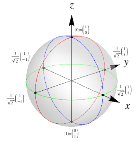
- de representatie van een uitwerking van een Hilbert space qubit in 3D ruimte
- de assen zijn (als altijd) arbitrair gekozen
- hier is de y-as de fase factor
- |u> and |d> zijn in Hilvert ruimte dus orthogonaal maar niet in 3d (daar een lineaire superpositie)
- synoniemen voor up zijn \(|u\rangle\) of \(|0\rangle\) of \(|+\rangle\)
14.4.1 Vrijheidsgraden van een qubit
- twee assen betekent 4 vrijheidsgraden
- maar dit worden er twee
- normalisatie vermindert met een
- phase indifference vermindert met een ander
- voor een individueel deeltje is de phase factor irrelevant: de uitkomst van een meting wordt er niet door beinvloed, en meer kan niet gekend worden
- voor >1 deeltje maakt de lokale (= relatieve) fase uit, maar de globale (= absolute) fase niet
- global phase indifference:
- \(|B \rangle = e^{i \theta} | A \rangle = e^{i \theta} \sum \limits_j \alpha_j | \lambda_j \rangle\)
- \(\langle B|B \rangle = \langle A e^{-i \theta}|e^{i \theta} A \rangle = \langle A | A \rangle\) want components uitschrijvend \(e^{i \theta}\alpha_j\) wordt vermenigvuldigd met conjugates \(\alpha^{*}_j e^{-i \theta}\) waarbij rotaties elkaar opheffen
14.5 Wavefunction
- als de staatvector van een systeem identitiek is aan een mogelijke uitkomst, zal de uitkomst met zekerheid in die staat verkeren
- de staatvector kan ook een kans op meerdere mogelijke uitkomsten bevattten ("in een Bloch sphere naar iets anders an up of down wijzen"): een lineaire "superpositie" van meerdere mogelijke uitkomsten: een golffunctie / wave function
- er treedt bij een meting dan een collaps van een superpositie naar een mogelijke uitkomst op: er wordt een eigenstate gekozen uit alle mogelijke eigenstates
- daarna verkeert het systeem in die eigenstate
- bijv. een qubit staatvector A in componenten (gelabeld naar de mogelijke uitkomsten, u or d) wordt zo genoteerd:
- \(| A \rangle = \alpha_u | u \rangle + \alpha_d | d \rangle\)
- de kolom met coefficienten (de alfa's) noem je de wave function
- een enkele coefficient uit de wave function kolom wordt ook wel "probability amplitude" genoemd (of "overlap" naar het inner product)
- de lengte van de vector langs de orthagonale as of eigenstate
- vermeningvuldiging met zijn eigen conjugaat heft het imaginaire deel op
- en daarna kwadrateren leidt tot positief getal: de kans op de uitkomst
- waarvoor dus geldt:
- \(\alpha_u = \langle u | A \rangle\)
- \(\alpha^*_u \alpha_u + \alpha^*_d \alpha_d = 1\) (normalisatie: <A|A> = 1)
- \(\langle u | d \rangle = 0\)
- \(P_u = \alpha^*_u \alpha_u = \langle A | u \rangle \langle u | A \rangle\)
- wave function kan genoteerd worden als
- \(\psi(a,b,c,...)\) waarbij \(a,b,c\) labels zijn zoals \(u\) en \(d\) (bijv. \(\alpha_u = \psi(u)\))
- identiek zijn dus
- \(| \psi \rangle = \sum \limits_j \alpha_j | \psi_j \rangle\) (an eigenfunction expansion), but also
- \(| \psi \rangle = \sum \limits_{a,b,c,....} \psi (a,b,c,...) | a,b,c,... \rangle\)
- \(\langle a,b,c,... | \psi \rangle\)
- \(| a,b,c,... \rangle\) is dan de bijbehorende set orthonormale basisvectoren
- "a,b,c,…" kunnen de bijbehorende eigenvalues zijn
- en \(A,B,C\) de defining communitative observables (zoals \(\sigma_z\) \(u\) and \(d\) definieert en dus \(\alpha_u\))
- het kwadraat is 1: \(\sum_{a,b,c...} \psi^*(a,b,c...) \psi (a,b,c...) = 1\)
- identiek zijn dus
- \(\psi(a,b)\), de coefficienten van staat psi als functie van a en b
- een kolom met de coefficienten (de α's, of componenten)
- \(\psi(a,b,c,...)\) waarbij \(a,b,c\) labels zijn zoals \(u\) en \(d\) (bijv. \(\alpha_u = \psi(u)\))
- note: soms wordt de staatvector een golffunctie genoemd (zoals 3 coordinaten een vector in een 3D ruimte "zijn")
14.6 "Preparing" a system
- na een collaps verkeert een systeem in een specifieke staat-vector
- dit maakt dat het leidt tot maximale kennis over het systeem
- en bijv. een vervolgmeting leidt tot dezelfde uitkomst
14.7 Eigenvector vergelijking
\(L | \lambda \rangle = \lambda | \lambda \rangle\)
14.7.1 The general principles
- principes:
- een meetbare grootheid (physical observable) wordt gerepresenteerd door een Hermitische operator (\(L\))
- de eigenvalues \(λ_i\) van de operator zijn de mogelijke uitkomsten
- in de eigenstate \(|λ_i \rangle\) is de uitkomst van een meting altijd \(λ_i\)
- zo niet (in superpositie) is \(P (λ_i) = \langle A | λ_i \rangle \langle λ_i | A \rangle\) de waarschijnlijkheid van de bijbehorende uitkomst
- met zekerheid te onderscheiden staten (|u> en |d> maar niet <u> en <r>) worden gerepresenteerd door orthogonale staatvectoren
- een degenerate state zijn twee ongelijke eigenvectoren met dezelfde eigenvalue
- dus, een operator heeft een aantal eigenvectoren en iedere eigenvector heeft een eigenvalue
14.7.2 Voetnoten
- beide vectoren \(|\lambda>\) zijn eigenvectoren
- aan de linkerkant: is de staat waarin het systeem verkeert voor de meting
- aan de rechterkant: de staat waarin het systeem na meting verkeert
- de eigenvalue λ (voor de vector aan de rechterkant, real getal):
- is het resultaat van de meting, en
- de factor waarmee de vector aan de linkerkant vermenigvuldigd wordt om de rechter te verkrijgen door deze uit te trekken
- negatieve eigenvalue spiegelt de vector
- de Hermitische operator is dus een "machine" die staten transformeert in een andere staat
- de letters zijn verwarrend gekozen: allemaal L's / lambda's maar \(L \neq \lambda \neq | \lambda \rangle\)
- wel houden ze alle verband met \(L\): \(L\) definieert hen, een operator is soort van een pakketje van eigenvectors en eigenvalues
- degeneratie moeilijk voor te stellen in de beeldbewerking
14.7.3 Vb met qubit
- \(\sigma_z | u \rangle = | u \rangle\)
- operator \(\sigma_z\) is de observable: de spin in de z-richting
- heeft twee eigenvalues: -1 en +1 (geen degeneracy), indien op eigenstate |u> toegepast levert +1 op
- \(\left( \begin{array}{c} 1 \;\;\;\;\; 0 \\ 0 \; -1 \end{array} \right)\) \(\left( \begin{array}{c} 1 \\ 0 \end{array} \right)\) = [+1] \(\left( \begin{array}{c} 1 \\ 0 \end{array} \right)\)
- \(\left( \begin{array}{c} 1 \;\;\;\;\; 0 \\ 0 \; -1 \end{array} \right)\) \(\left( \begin{array}{c} 0 \\ 1 \end{array} \right) = \left( \begin{array}{c} 0 \\ -1 \end{array} \right)\) = -[1] \(\left( \begin{array}{c} 0 \\ 1 \end{array} \right)\)
14.7.4 Vb expectation value
- \(\langle L \rangle = \langle A | L | A \rangle = \sum \limits_i \lambda_i P(\lambda_i)\) where \(\langle A | L | A \rangle\) is \(L | A \rangle\) multiplied with \(\langle A |\)
- voorbeeld:
- \(|r \rangle = \frac{1}{\sqrt 2}|u \rangle + \frac{1}{\sqrt 2}|d \rangle\)
- \(\sigma_z |r \rangle = \frac{1}{\sqrt 2} \sigma_z |u \rangle + \frac{1}{\sqrt 2} \sigma_z |d \rangle\)
- \(\sigma_z |r \rangle = \frac{1}{\sqrt 2}|u \rangle - \frac{1}{\sqrt 2}|d \rangle = \left( \begin{array}{c} \frac{1}{\sqrt 2} \\ - \frac{1}{\sqrt 2} \end{array} \right)\)
- \(\langle r| \sigma_z |r \rangle = (\frac{1}{\sqrt 2}, \frac{1}{\sqrt 2}) \left( \begin{array}{c} \frac{1}{\sqrt 2} \\ - \frac{1}{\sqrt 2} \end{array} \right) = \frac{1}{2} - \frac{1}{2} = 0\)
14.8 Pauli matrices
- \(\sigma_z = \left( \begin{array}{c} 1 \; \; \; \; 0 \\ 0 \; \; {-1} \end{array} \right)\)
- \(\sigma_x = \left( \begin{array}{c} 1 \; \; 0 \\ 0 \; \; 1 \end{array} \right)\)
- \(\sigma_y = \left( \begin{array}{c} 0 \; \; \; \; i \\ -i \; \; 0 \end{array} \right)\)
- \(I = \left( \begin{array}{c} 1 \; \; 0 \\ 0 \; \; 1 \end{array} \right)\)
- algemeen \(\left( \begin{array}{c} r \; \; \; \; w \\ w^* \; \; r \end{array} \right)\)
- iedere Hermitische operator L kan uitgedrukt worden als \(L = a \sigma_x + b \sigma_y + c \sigma_z + d I\)
- I is saai: 1 is de enige eigenstaat en alle vectoren eigenvectors
14.9 Matrix
- \(M | A \rangle = |B \rangle\)
- the operator M is a machine that changes states into other states, transforms
- M is an operator and its components m are a matrix (in a orthonormal basis), mark the capitals (vectors) and non-capitals (components)
- components are defined by \(m_{jk} = \langle j|M|k\rangle\)
- in matrix notation: \(\left( \begin{array}{c} m_{11} \: m_{12} \: m_{13} \\ m_{21} \: m_{22} \: m_{23} \\ m_{31} \: m_{32} \: m_{33} \end{array} \right) \left( \begin{array}{c} \alpha_1 \\ \alpha_2 \\ \alpha_3 \end{array} \right) = \left( \begin{array}{c} \beta_1 \\ \beta_2 \\ \beta_3 \end{array} \right)\) or \(\sum \limits_j m_{kj} \alpha_j = \beta_k\)
- dus \(\beta_1\) wordt berekend door de bovenste rij te vermenigvuldigen met alle \(\alpha\)'s, de eerste van de rij met de eerste van de kolom, etc: \(\beta_1 = m_{11} \alpha_{1} + m_{12} \alpha_2 + m_{13} \alpha_3\)
- mark m11 is a complex number, the subscripts for a matrix are in the order yx
- the operator usually represented as a NxN matrix, which allows multiplication with a ket without conjugation
- rules
- Mz|A> = z|B>
- M{|A> + |B>} = M|A> + M|B>
- matrix calculation
- addition / subtraction: https://www.studypug.com/algebra-help/adding-and-subtracting-matrices
14.10 <A|M|B>
- op te lossen door
- transformatie, in principe van B
- inner product met A
- interpretatie
- positie in matrix: complex getal
- indien A=B
- <A|L|A> = Tr |A><A| L
- <A|L|A> = <L>
- de expectation value: deze zitten dus in de diagonaal van een operatormatrix
- en indien het een eigenvector betreft (altijd bij een projectie-operator): de eigenvalues
14.11 Hermitic operator
- a linear operator
- a Hermitic operator is equivalent to its own conjugate: \(L = L \dagger\)
- \(L \dagger = [M^T]^* \Rightarrow m_{ji} = m^*_{ij}\), the definition of a dagger
- note the difference in subscripts: the matrix is mirrored and conjugated
- M|A> = |B> → <A|M† = <B|
14.12 Kronecker product
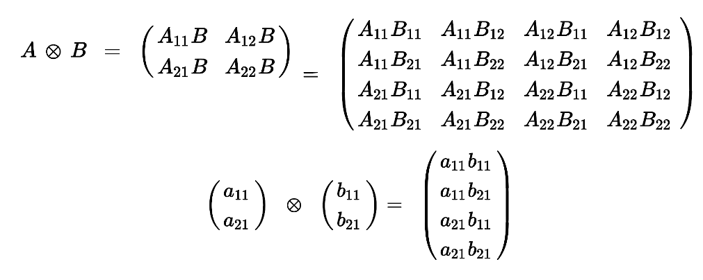
- Kronecker multiplication: tensor product of matrices
- m × n matrix and a p × q matrix is an mp × nq matrix.
- Kronecker-formule
- Voorbeeld Kronecker
14.13 Schrodinger
- U is de operator die de transformatie toont, \(\psi(t) = U(t) | \psi(0) \rangle\)
- de ontwikkeling van een staat in de tijd is dus wel deterministisch
- uit behoud van onderscheid (\(\langle \psi(0) | \phi(0) \rangle = 0 \Rightarrow \langle \psi(t) | \phi(t) \rangle = 0\))
- volgt \(U^\dagger U = I\) (en \(\Rightarrow U^\dagger = U\))
- "time evolution is unitary"
- H is the quantum Hamiltonian
- een Hermitische operator en "unitary"
- zijn eigenvalues de energie van een systeem
- \(\frac{\partial | \psi \rangle}{\partial t} = \frac{-i}{\hbar} H | \psi \rangle\) is de algemene (of tijd-afhankelijke) Schrodinger (TAS) vergelijking tenzij H van t afhankelijk is1
- \(H|E_j \rangle = E_j | E_j \rangle\) is de tijd-onafhankelijke Schrodinger (TOS) vergelijking
- om de Schrodinger vergelijking op te lossen
- vindt de Hamiltoniaan
- maak een initiele staat: \(|\psi_0\rangle\)
- vindt de eigenvalues en eigenvectors door de TOS op te lossen, bijv. door een golffunctie en/of operator in te vullen
- stel de initiele coefficienten vast: \(|\psi_0\rangle = \sum \limits_j \alpha_j(0) | E_j \rangle\)
- zet hem om naar een tijdafhankelijke vergelijking \(|\psi\rangle = \sum \limits_j \alpha_j(0) e^{-\frac{i}{\hbar}E_jt}|E_j\rangle\)
14.14 Commutator
- LH - HL = [L,H] waarbij [] de commutator is en waarvoor geldt [L, M] = -[M, L]
- zoals in de beeldbewerking maakt volgorde van operator uit: LH-HL is not per definition zero
- <[L,H]> wordt vaak genoteerd als [L,H], zoals in volgende voorbeeld
- functies
- \(\frac{dL}{dt} = -\frac{i}{\hbar} [L, H]\) 2
- de algebra lijkt op die van Poisson Brackets: de wiskundige connectie is: [F,G] = i ℏ {F, G}
- dus op een menselijke schaal is het effect verwaarloosbaar
- two observables commute if there is a complete basis of simultaneous eigenvectors
- if they do not
- one is always uncertain as
- one can be certain (if the system is in an eigenvector) but
- that vector will not be the eigenvector of the non-commuting operator
- complete basis of simultaneous eigenvectors
- \(L|\lambda_i, \mu_A \rangle = \lambda_i|\lambda_i, \mu_a \rangle\)
- \(M|\lambda_i, \mu_A \rangle = \mu_i|\lambda_i, \mu_a \rangle\)
- we will leave out the subscripts in the future
- \([L,M] | \lambda, \mu \rangle = 0\) can be proven, where 0 is the zero vector, a operator that annihilates every member is the zero operator
- if they do not
- Q is behouden indien een gesloten systeem indien het "commute" met de Hamiltoniaan.
- als QH = HQ dan is [Q, H] = 0, of "Q and H commute"
- \(\frac{dL}{dt} = -\frac{i}{\hbar} [L, H]\) 2
14.14.1 Voorbeeld
- find the Hamiltonian: e.g. \(H = \vec{\sigma} \cdot \vec{B} = \sigma_x B_x + \sigma_y B_y + \sigma_z B_z\)
- make it simple (parallel to z): \(H = \frac{\hbar \omega}{2} \sigma_z\)
- get the commutator to find the derivative of an observable: \(\langle \dot{\sigma_x} \rangle = - \frac{i}{\hbar} \langle[\sigma_x, H] \rangle\), etc.
- fill the Hamiltonian in the derivative: \(\langle \dot{\sigma_x} \rangle = - \frac{i \omega}{2} \langle[\sigma_x, \sigma_z] \rangle\)
- use the Pauli matrices: \([\sigma_x, \sigma_z] = 2i \sigma_z\)
- thus: \(\langle \dot{\sigma_x} \rangle = - \omega \langle \sigma_y \rangle\)
14.15 Heisenberg
14.15.1 Standard deviation
- \(\bar{A} = A - \langle A \rangle\) men trekke de expectation value af van operator A
- \(\bar{A} = A - I \langle A \rangle\) ieder real getal is een operator als je hem met I vermenigvuldigt
- effect is dezelfde probability distribution: \(\langle A \rangle = \sum \limits_a aP(a)\) (waarbij a de eigenvalues zijn)
- maar met een veschuiving van de eigenvalues: \(\bar{a} = a - \langle A \rangle\)
- "onzekerheid" Δ: \((\Delta A)^2 = \sum \limits_a \bar{a}^2 P(a) = \langle \psi | \bar{A}^2 | \psi \rangle\)
- als de expectation value nul is: \((\Delta A)^2 = \langle \psi | A^2 | \psi \rangle\)
14.15.2 Cauchy-Schwartz
- de lange zijde van een driehoek is minder de som van de andere twee
- want het kortste pad is de rechte lijn
- dit geldt ook voor driehoeken van vectoren en in ieder aantal dimensies en in een vectorruimte
- if the length of the vector is defined as the square root of the vector’s inner product with itself
- \(|\vec{X}| + |\vec{Y}| \geq | \vec{Z} |\)
- this leads to \(2|X||Y| \geq | \langle X | Y \rangle + \langle Y | X \rangle |\)
- als \(|X \rangle = A | \psi \rangle\) en \(|Y \rangle = iB | \psi \rangle\) dan volgt:
- \(\Delta A \Delta B \geq \frac{1}{2} | \langle \psi | [A,B] | \psi \rangle |\)
14.16 Projectie-operator
- \(|\phi\rangle \langle \psi|\)
- lineaire operator
- projection operator: \(|\phi\rangle \langle \phi|\)
- \(|\phi\rangle \;\; \langle \phi|A\rangle\) is always proportional to \(|\phi\rangle\)
- Hermitisch
- eigenvalues are either 0 or 1
- de vector van de projectie-operator heeft eigenvalue 1 (\(|\psi\rangle \langle\psi| \; |\psi\rangle = |\psi\rangle\))
- iedere orthogonale vector eigenvalue 0
- de trace (de som van de diagonaal, dus de som van de eigenvalues) is 1: \(Tr L = \sum \limits_i \langle i|L|i \rangle\)
- het kwadraat is gelijk aan de projectie-operator zelf (normalisatie)
- all projection operators of a system added results in I: \(\sum \limits_i = |i\rangle\langle|i| = I\)
- \(\langle\psi|L|\psi\rangle = Tr |\psi\rangle \langle\psi| L\)
14.17 Density matrix
- \(\langle L \rangle = Tr \rho L\)
- \(\rho = P_1|\phi_1\rangle\langle\phi_1 + P_2|\phi_2\rangle\langle\phi_2 +\)…
- daadwerkelijk matrix indien \(\rho_{aa'} = \langle a | \rho | a' \rangle\)
- en geldt: \(\langle L \rangle\)
14.18 Entanglement
14.18.1 Tensor product
- \(S_{AB} = S_A \otimes S_B\)
- \(N_{AB}= N_A N_B\), aantal (orthogonale) dimensies (aantal opties, twee bij een munt)
- benaming voor staten, A is een munt (H/T) en B een dobbelsteen, let op, andere ketnotatie voor A en B omdat ze niet opgeteld kunnen worden
- \(|H\} \otimes |4 \rangle\)
- \(|H\}|4 \rangle\)
- \(|H4 \rangle\) waarbij arbitrair A voor B komt
- of algemeen \(|ab \rangle\) en voor een tweede staat \(|a'b' \rangle\)
- het dubbel gelabelde systeem-van-twee is een enkele staat dat wel opgeteld kan worden
- \(\langle ab | a'b' \rangle = \delta_{aa'}\delta_{bb'}\) alleen als het complete label overeenkomt is de staat niet orthogonaal
- de eigenfunctie expansie van een dubbele staat is \(\psi \rangle = \sum \limits_{a,b} \psi(a,b) | ab \rangle\)
14.18.2 Klassieke entanglement
- aan twee mensen twee afgedekte munten geven, een kop en een munt
- tegelijkertijd de munten bekijken
14.18.3 Entanglement statistics
- correlatie: \(\langle \sigma_A \sigma_B \rangle - \langle \sigma_A \rangle \langle \sigma_B \rangle\), indien niet-nul gecorreleerd
- \(\langle \sigma_A \rangle = 0\)
- \(\langle \sigma_B \rangle = 0\)
- \(\langle \sigma_A \sigma_B \rangle = -1\)
- factorisatie: \(P(a,b) = P_A(a) P_B(b)\) indien ze niet-gecorreleerd zijn
14.18.4 Quantum entanglement
- NB τx bepaald op "up"-staat is vaak de x-up staat
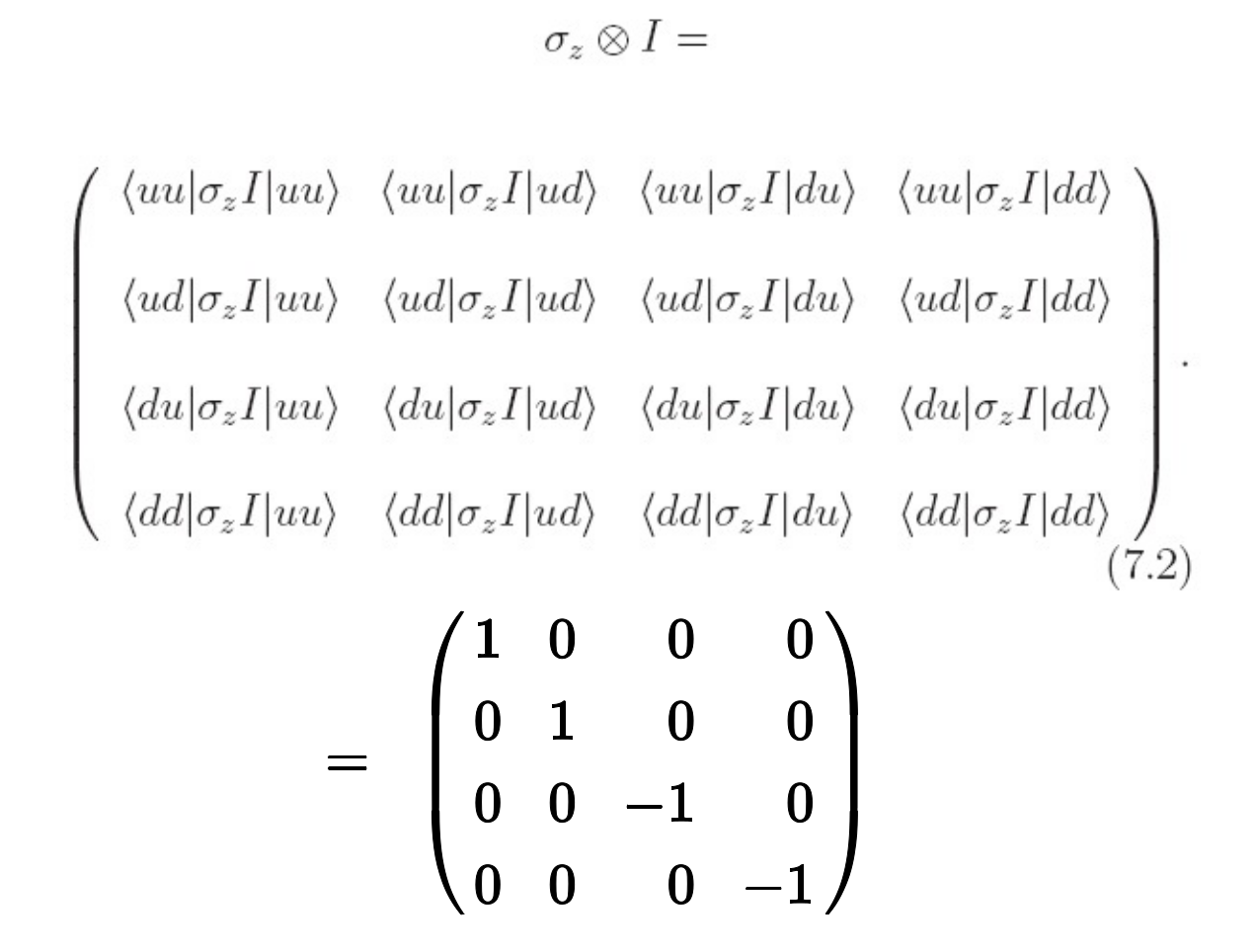
- twee spin operatoren, σ voor A en τ voor B: de operator voor A negeert simpelweg de B-staat, en vice-versa
- \(\sigma_z | du \rangle = - |du \rangle\) is: \((\sigma_z \otimes I)(|d \rangle \otimes |u \rangle) = (\sigma_z|d \rangle \otimes I | u \rangle) = (-|d \rangle \otimes | u \rangle )\)
- productstaat: σ en τ hangen niet samen
- \(\alpha_u|u\} + \alpha_d|d\}\)
- \(\beta_u|u\rangle + \beta_d|d\rangle\)
- \(\alpha_u^* \alpha_u + \alpha_d^* \alpha_d = 1\)
- \(\beta_u^* \beta_u + \beta_d^* \beta_d = 1\)
- |product state⟩ = ( \(\alpha_u|u\} + \alpha_d|d\} ) \otimes (\beta_u|u\rangle + \beta_d|d\rangle)\)
- 4 vrijheidsgraden freedom (4 complexe getallen - normalisatie vereiste - globale fase)
- \(\langle\sigma_z\rangle + \langle\sigma_x\rangle + \langle\sigma_y\rangle = 1\) het spin polarisatie principe
- (maximaal) entangled state
- e.g. singlet staat \(|sing\rangle = \frac{1}{\sqrt{2}}(|ud \rangle - |du \rangle)\)
- \(\psi_{uu}^* \psi_{uu} + \psi_{ud}^*\psi_{ud} + \psi_{du}^* \psi_{du} + \psi_{dd}^*\psi_{dd} = 1\)
- 6 vrijheidsgraden
- \(\langle\sigma_z\rangle = \langle\sigma_x\rangle = \langle\sigma_y\rangle = 0\) (wat gebeurt er na een collaps?)
- een entangled state is een complete beschrijving van het gecombineerde systeem, maar ondanks dat de staat volledig bekend is, kan er niets meer over bekend zijn: men kan niets weten over de individuele onderdelen
- gecombineerde operator
- alle operatoren van een tensorproduct "commute" en kunnen samen gemeten worden
- \(\tau_z\sigma_z\) is de product van de metingen van σ en τ
- \(\tau_z\sigma_z | sing \rangle = -|sing \rangle\): ze hebben altijd de tegenovergestelde uitkomst
- \(\tau_y\sigma_y | sing \rangle = -|sing \rangle\): wat niet meteen evident is als je naar \(|sing\rangle\) kijkt
- \(\tau_z\sigma_z\) heeft \(|sing\rangle\) als een eigenvector met -1 als eigenvalue
- \(\vec{\sigma} \cdot \vec{\tau} = \sigma_x \tau_x + \sigma_y \tau_y + \sigma_z \tau_z\)
- kan niet door de individuele spin componenten te bepalen: they do not commute
- zekunnen ook niet los gemeten worden
- het is soms de gecombineerde Hamiltoniaan van een atoom nabij een andere in een kristal
- \(|sing\rangle\) is de eigenvector van \(\vec{\sigma} \cdot \vec{\tau}\)
- dit geldt ook voor de triplet staten, die zo heten omdat ze ook een eigenvector zijn met een andere gedegenereerde eigenvalue
- ud+du
- uu+dd
- uu-dd
15 Strange quantum effects
15.1 Measuring spin
- If spin was a normal vector, a measurement a right angle should result in zero. It only does so on average.
- Measuring spin in one direction destroys information on another component.
- One can never know two orthogonal components of spin simultaneously in a reproducible manner.
15.2 Quantum mechanical logic
- Two propositions
- The z component of spin is +1
- The x component of spin is +1
- The z component is +1 and z and x are determined sequentially.
- The classical meaning of the Boolean logic of (1 OR 2) changes, as in 1/4 the results is false if we reverse the order of testing: (1 OR 2) is different from (2 OR 1).
- The classical (1 AND 2) even becomes meaningless as this is not confirmable.
15.3 Entanglement
16 Verwijderd
Footnotes:
1
Solving the Time-dependent Schrodinger
- \(| \psi(t) \rangle = \sum \limits_j \alpha_j(t) | E_j \rangle\)
- \(\sum \limits_j \dot{\alpha}_j(t) | E_j \rangle = - \frac{i}{\hbar} H \sum \limits_j \alpha_j(t) | E_j \rangle\) combination with time-dependent equation
- \(\sum \limits_j \dot{\alpha}_j(t) | E_j \rangle = - \frac{i}{\hbar} \sum \limits_j E_j \alpha_j(t) | E_j \rangle\) combination with time-independent equation
- \(\sum \limits_j [ \dot{\alpha}_j(t) + \frac{i}{\hbar} E_j \alpha_j(t) ] | E_j \rangle = 0\)
- \(\frac{d \alpha_j (t)}{dt} = - \frac{i}{\hbar} E_j \alpha_j(t)\)
- thus there is a relation between time and energy
- \(| \psi (t) \rangle = \sum \limits_j \alpha_j(0) e^{-\frac{i}{\hbar}E_jt} | E_j \rangle\) en \(\alpha_j(0) = \langle E_j | \psi(0) \rangle\)
- \(| \psi (t) \rangle = \sum \limits_j | E_j \rangle \langle E_j | \psi(0) \rangle e^{-\frac{i}{\hbar}E_jt}\)
- \(P_\lambda(t) = | \langle \lambda | \psi (t) \rangle |^2\)
2
differentiating an observable:
- \(\frac{d}{dt} \langle \psi(t) | L | \psi(t) \rangle = \langle \dot{\psi}(t)|L|\psi(t) \rangle + \langle \psi(t)|L|\dot{\psi(t)} \rangle = \frac{i}{\hbar} \langle \psi(t)|HL|\psi(t) - \frac{i}{\hbar} \langle \psi(t)|LH|\psi(t) \rangle = \frac{i}{\hbar} \langle \psi(t) | \; [HL-LH] \; | \psi(t) \rangle\)
- \(\frac{d}{dt} \langle L \rangle = \frac{i}{\hbar} \langle [H,L] \rangle\)